フォン・ノイマン＝ベルナイス＝ゲーデル集合論

数学基礎論において、フォン・ノイマン＝ベルナイス＝ゲーデル集合論 (NBG) とはツェルメロ＝フレンケル集合論＋選択公理 (ZFC)の保存拡大である公理的集合論である。NBGでは、量化子の範囲を集合に限定した論理式によって定義される集合の集まりとして、クラスの概念を導入する。NBGは、すべての集合というクラスやすべての順序数というクラスといった、集合よりも大きいクラスを定義できる。モース＝ケリー集合論 (MK) は量化子の範囲がクラスである論理式によるクラスの定義を許容する。NBGは有限公理化できる一方、ZFCやMKではできない。

NBGのキーとなる定理はクラスの存在定理である。クラスの存在定理は、量化子の範囲を集合に限定した論理式それぞれに対して、論理式を満たす集合からなるクラスの存在を述べる。クラスは、クラスの論理式を一つずつ構築することで構成される。すべての集合論的な論理式は2種類の原子論理式（所属関係と等式）と有限個の論理記号から構築されるため、論理式を満足するクラスを構築するには有限個の公理があればよい。NBGが有限公理化できるのは、こうした理由による。クラスは他の概念の構築にも用いられ、集合論的パラドックスへの対処や、ZFCの選択公理より強い大域選択公理（英語版）の説明に用いられる。

ジョン・フォン・ノイマンは1925年に集合論にクラスを導入した。彼の理論の原始概念（英語版）は関数と引数であった。これらの概念を用いて、フォン・ノイマンはクラスと集合を定義した。^[1] パウル・ベルナイスはクラスと集合を原始概念とすることで、フォン・ノイマンの理論を再定式化した。^[2] クルト・ゲーデルは、選択公理の相対的無矛盾性の証明と一般連続体仮説を用いてベルナイスの理論を単純化した。^[3]

集合論におけるクラス

クラスの使用例

NBGにおいてクラスはいくつかの使用例がある：

• クラスによって集合論を有限公理化する。^[4]
• "非常に強い形の選択公理"を表現するのに用いられる。^[5]—すなわち、大域選択公理（英語版）のことである。大域選択公理の内容は以下の通り：すべての空でない集合 ${\displaystyle x}$ に対して ${\displaystyle G(x)\in x}$ である、すべての空でない集合のクラス上に定義された大域選択関数 ${\displaystyle G}$ が存在する。大域選択公理はZFCの選択公理よりも強い。ZFCの選択公理の内容は以下の通り：任意の空でない集合の集合 ${\displaystyle s}$ について、すべての ${\displaystyle x\in s}$ に対して ${\displaystyle f(x)\in x}$ である ${\displaystyle s}$ 上の選択関数（英語版） ${\displaystyle f}$ が存在する。^{[注釈 1]}
• 集合でないクラスが存在することを認めると、集合論的パラドックスは解決される。例えば、すべての順序数のクラス ${\displaystyle Ord}$ を集合であると仮定する。すると、 ${\displaystyle Ord}$ は ${\displaystyle \in }$ で整列された推移的集合となる。すなわち、定義から ${\displaystyle Ord}$ は順序数である。したがって、 ${\displaystyle Ord\in Ord}$ であるが、これは ${\displaystyle Ord}$ が ${\displaystyle \in }$ で整列されていることに矛盾する。したがって、 ${\displaystyle Ord}$ は集合ではない。集合ではないクラスを真のクラスと呼ぶため、 ${\displaystyle Ord}$ は真のクラスである。^[6]
• 真のクラスは集合などの作成に便利である。 大域選択公理と一般連続体仮説の相対的非矛盾性の証明において、ゲーデルは構成可能集合を作るのに真のクラスを用いた。ゲーデルはすべての順序数のクラス上の関数を構成した。すなわち、各順序数について、構成済の集合に対して集合を作る処理を適用することで構成可能集合を作った。構成可能集合はこの関数の像である。^[7]

公理型とクラス存在定理

ZFCの言葉にクラスが加えられれば、ZFCをクラス付きの集合論に変換するのが容易になる。まず、クラス解釈の公理型を加える。この公理型は以下の通り：量化子の範囲を集合に限定したすべての論理式 ${\displaystyle \phi (x_{1},\ldots ,x_{n})}$ に対して、論理式を満たす ${\displaystyle n}$-組からなるクラス ${\displaystyle A}$ が存在する—すなわち、 ${\displaystyle \forall x_{1}\cdots \,\forall x_{n}[(x_{1},\ldots ,x_{n})\in A\iff \phi (x_{1},\ldots ,x_{n})]}$ である。すると置換公理はクラスを用いる一つの公理で置き換えられる。最後に、ZFCの外延性の公理はクラスを扱う形に修正される：2 つのクラスが同じ元を持つならば、それらのクラスは等しい。ほかのZFCの公理は修正されない。^[8]

この理論は有限公理化されない。ZFCの置換公理型は一つの公理で置き換えられるが、クラス解釈の公理はZFCに導入されていないからである。

この理論を有限個の公理で構築するには、まずクラス解釈の公理を有限個のクラス外延性の公理で置き換える。するとこれらの公理は、公理系中のどの公理をも含意するクラス存在定理に用いられる。^[8] この理論の証明には 7 つのクラス存在公理があれば十分である。これらのクラス存在公理は、論理式の構成から論理式を満たすクラスの構成へ変換するのに用いられる。

NBGの公理化

クラスと集合

NBGにはクラスと集合という 2 種類の対象がある。直感的には、どの集合も同時にクラスである。これを公理化する方法は 2 通り存在する。ベルナイスは 2 ソートの多ソート論理を用いた。^[2] ゲーデルはソートの代わりに原始述語を用いた： ${\displaystyle {\mathfrak {Cls}}(A)}$ を「 ${\displaystyle A}$ はクラスである」ことを、 ${\displaystyle {\mathfrak {M}}(A)}$ を「 ${\displaystyle A}$ は集合である」ことを表す述語とする（ドイツ語では集合は Menge である)。ゲーデルは「すべての集合はクラスである」という公理と、「クラス ${\displaystyle A}$ がクラスの元であれば、 ${\displaystyle A}$ は集合である」という公理を導入した。^[9] 述語はソートの回避のためによく使われる。 エリオット・メンデルソン (Elliott Mendelson) はゲーデルの考え方を元に、全てをクラスとした上で、 ${\displaystyle \exists C(A\in C)}$ を表す述語 ${\displaystyle M(A)}$ で集合を表すことで修正した。^[10] この修正によって、ゲーデルのクラス述語と 2 つの公理は不要になる。

ベルナイスの 2 ソートのアプローチのほうが最初は自然に見えるかもしれないが、こちらは複雑な理論になる。^{[注釈 2]} ベルナイスの理論では、どの集合も 2 種類の表現を持つ：一つは集合として、もう一つはクラスとしてである。同時に、2 つの 帰属関係がある：一つは "∈" で表される 2 つの集合間の関係、もう一つは "η" で表される集合とクラスの間の関係である。^[2] 異なるソートの変数は議論領域中で互いに素な部分領域の元となるため、この冗長性は多ソート論理に必要になる。

これらの 2 つのアプローチで証明できるものは変わらないが、証明の書かれ方は変わってくる。ゲーデルのアプローチでは、 ${\displaystyle A}$ と ${\displaystyle C}$ がクラスであるとき ${\displaystyle A\in C}$ は有効な表現である。ベルナイスのアプローチではこの表現は意味をなさない。しかし、 ${\displaystyle A}$ が集合であれば、等価な表現が存在する： 集合とクラスが同じ集合を元に持つならば、「集合 ${\displaystyle a}$ はクラス ${\displaystyle A}$ を代表する」と定義する。—すなわち、 ${\displaystyle \forall x(x\in a\iff x\;\eta \;A)}$。集合 ${\displaystyle a}$ がクラス ${\displaystyle A}$ を代表するという表現 ${\displaystyle a\;\eta \;C}$ は、ゲーデルの ${\displaystyle A\in C}$ と等価である。^[2]

本記事ではゲーデルのアプローチのメンデルソンによる修正版を用いて説明する。これは、NBG は等式を含む一階述語論理における公理系であることを意味し、原始概念（英語版）はクラスと帰属関係のみであることを意味する。

外延性の公理と対の公理の定義

集合は、少なくとも 1 つのクラスに属するクラスである： ${\displaystyle \exists C(A\in C)}$ のとき、かつそのときに限り ${\displaystyle A}$ は集合である。 集合でないクラスは真のクラスと呼ぶ：${\displaystyle \forall C(A\notin C)}$ のとき、かつそのときに限り ${\displaystyle A}$ は真のクラスである。^[12] したがって、どのクラスも集合または真のクラスであり、両方同時に当てはまることはない。

ゲーデルは大文字の変数をクラス上の変数、小文字の変数を集合上の変数とした。^[9] また、ゲーデルは、すべての集合からなるクラス上に定義された関数や関係を含む特定のクラスは、大文字から始まる名前で表した。本記事ではゲーデルのこの表記法に従う。すると以下のように書ける：

以下の公理と定義はクラス存在定理の証明に必要である。

外延性の公理.  2 つのクラスが同じ元を持っていれば、それらは等しい。

${\displaystyle \forall A\,\forall B\,[\forall x(x\in A\iff x\in B)\implies A=B]}$ ^[13]

この公理はZFCの外延性の公理をクラスに一般化したものである。

対の公理.  ${\displaystyle x}$ と ${\displaystyle y}$ が集合であれば、元が ${\displaystyle x}$ と ${\displaystyle y}$ のみである集合 ${\displaystyle p}$ が存在する。

${\displaystyle \forall x\,\forall y\,\exists p\,\forall z\,[z\in p\iff (z=x\,\lor \,z=y)]}$ ^[14]

ZFCのように、外延性の公理は集合 ${\displaystyle p}$ がただ一つであることを含意する。これによって ${\displaystyle \{x,y\}}$ という表記ができる。

順序対は以下のように定義される。

${\displaystyle (x,y)=\{\{x\},\{x,y\}\}}$

対は順序対を使って再帰的に定義される：

${\displaystyle (x_{1})=x_{1},}$

${\displaystyle {\text{For }}n>1\!:(x_{1},\ldots ,x_{n-1},x_{n})=((x_{1},\ldots ,x_{n-1}),x_{n}).}$^{[注釈 3]}

クラス存在公理と正則性公理

クラス存在公理はクラス存在定理を証明するのに用いる：集合のみを量化する ${\displaystyle n}$ 個の集合の自由変数に関するすべての論理式について、その論理式を満たす ${\displaystyle n}$-組のクラスが存在する。以下の例は、関数のクラスと合成関数を構築するクラスの 2 つのクラスから始める。この例はクラス存在定理を証明するのに必要な、クラス存在公理を導出する手法を説明する。

例 1:  クラス ${\displaystyle F}$ と ${\displaystyle G}$ が関数であるならば、合成関数 ${\displaystyle G\circ F}$ は以下の論理式で定義される： ${\displaystyle \exists t[(x,t)\in F\,\land \,(t,y)\in G].}$ この論理式は 2 つの集合に関する自由変数 ${\displaystyle x}$ と ${\displaystyle y}$ を持つため、クラス存在定理から以下の順序対のクラスの存在が導かれる： ${\displaystyle G\circ F\,=\,\{(x,y):\exists t[(x,t)\in F\,\land \,(t,y)\in G]\}.}$ この論理式は論理積 ${\displaystyle \land }$と存在記号 ${\displaystyle \exists }$を使って簡潔に構築されているので、簡潔な論理式を表すクラスを使って${\displaystyle \land }$ と ${\displaystyle \exists }$ を含む論理式を表すクラスを生成するクラス演算が必要である。${\displaystyle \land }$の論理式を表すクラスを作るには、${\displaystyle x\in A\cap B\iff x\in A\land x\in B}$であることから共通部分を用いる。${\displaystyle \exists }$の論理式を表すクラスを作るには、${\displaystyle x\in Dom(A)\iff \exists t[(x,t)\in A].}$であることから領域を用いる 共通部分を求める前に、${\displaystyle F}$ と ${\displaystyle G}$ にそれぞれ含まれる組において、共通した変数を持つように他の要素が必要になる。元 ${\displaystyle y}$ を ${\displaystyle F}$ の組に、 元 ${\displaystyle x}$ を ${\displaystyle G}$ の組に加える： $${\displaystyle F'=\{(x,t,y):(x,t)\in F\}\,}$$ $${\displaystyle \,G'=\{(t,y,x):(t,y)\in G\}}$$ ${\displaystyle F'}$ の定義において、変数 ${\displaystyle y}$ は ${\displaystyle (x,t)\in F}$ で制限されないため、 ${\displaystyle y}$ の定義域はすべての集合のクラス ${\displaystyle V}$ 上になる。同様に、${\displaystyle G'}$ の定義において、変数 ${\displaystyle x}$ の定義域も ${\displaystyle V}$ 上になる。ここで与えられたクラスの組に（${\displaystyle V}$上の）追加の元を加える公理が必要になる。 次に、共通部分をとる準備として、変数を同じ順序で並べる： $${\displaystyle F''=\{(x,y,t):(x,t)\in F\}\,}$$ $${\displaystyle \,G''=\{(x,y,t):(t,y)\in G\}}$$ ${\displaystyle F'}$ から ${\displaystyle F''}$ および ${\displaystyle G'}$ から ${\displaystyle G''}$ へは、2 種類の巡回が必要になる。ゆえに、組の元の巡回を扱う公理が必要になる。 ${\displaystyle F''}$ と ${\displaystyle G''}$ の共通部分は ${\displaystyle \land }$ で表現される： $${\displaystyle F''\cap G''=\{(x,y,t):(x,t)\in F\,\land \,(t,y)\in G\}}$$ ${\displaystyle (x,y,t)}$ は ${\displaystyle ((x,y),t)}$ として定義されるので、${\displaystyle F''\cap G''}$ の領域は ${\displaystyle \exists t}$ で表現され、合成関数を生成する： $${\displaystyle G\circ F=Dom(F''\cap G'')=\{(x,y):\exists t((x,t)\in F\,\land \,(t,y)\in G)\}}$$ したがって、共通部分および領域の公理が必要である。

クラス存在公理は 2 つのグループに分かれる：述語に関する公理と、対に関する公理である。前者のグループには 4 つの公理が、後者のグループには 3 つの公理が含まれる。^{[注釈 4]}

述語に関する公理：

帰属.  1番めの要素が 2 番めの要素の元になるような順序対すべてを含むクラス ${\displaystyle E}$ が存在する。

${\displaystyle \exists E\,\forall x\,\forall y\,[(x,y)\in E\iff x\in y]\!}$ ^[18]

共通部分（連言）.  任意の 2 つのクラス ${\displaystyle A}$ と ${\displaystyle B}$ に対して、 ${\displaystyle A}$ と ${\displaystyle B}$ にそれぞれ属する集合のみからなるクラス ${\displaystyle C}$ が存在する。

${\displaystyle \forall A\,\forall B\,\exists C\,\forall x\,[x\in C\iff (x\in A\,\land \,x\in B)]}$ ^[19]

補集合（否定）.  任意のクラス ${\displaystyle A}$ に対して、 ${\displaystyle A}$ に属さない集合のみからなるクラス ${\displaystyle B}$ が存在する。

${\displaystyle \forall A\,\exists B\,\forall x\,[x\in B\iff \neg (x\in A)]}$ ^[20]

領域（存在量化子）.  任意のクラス ${\displaystyle A}$ に対して、 ${\displaystyle A}$ の順序対の最初の要素からなるクラス ${\displaystyle B}$ が存在する。

${\displaystyle \forall A\,\exists B\,\forall x\,[x\in B\iff \exists y((x,y)\in A)]}$ ^[21]

外延性の公理より、共通部分公理におけるクラス ${\displaystyle C}$ と補集合公理および領域公理におけるクラス ${\displaystyle B}$ はそれぞれただ一つ定まる。これらはそれぞれ以下のように表現される：${\displaystyle A\cap B,}$ ${\displaystyle \complement A,}$ and ${\displaystyle Dom(A).}$^{[注釈 5]} 一方、帰属公理はクラス ${\displaystyle E}$ 上の順序対の集合のみを規定するため、外延性の公理は帰属公理におけるクラス ${\displaystyle E}$ には適用できない。

最初 3 つの公理は空クラスおよびすべての集合のクラスの存在を含意する：帰属公理はクラス ${\displaystyle E}$ の存在を含意する。共通部分公理および補集合公理は、空クラスである ${\displaystyle E\cap \complement E}$ の存在を含意する。外延性の公理により、このクラスはただ一つ定まり、これを ${\displaystyle \emptyset }$ で表す。 ${\displaystyle \emptyset }$ の補集合はすべての集合のクラス ${\displaystyle V}$ であり、これも外延性の公理からただ一つ定まる。すると、 ${\displaystyle \exists C(A\in C)}$ を表す集合述語 ${\displaystyle M(A)}$ は、クラスを量化することなく ${\displaystyle A\in V}$ と再定義される。

対に関する公理：

${\displaystyle V}$ の直積.  任意のクラス ${\displaystyle A}$ に対して、最初の要素が ${\displaystyle A}$ に属する順序対からなるクラス ${\displaystyle B}$ が存在する。

${\displaystyle \forall A\,\exists B\,\forall u\,[u\in B\iff \exists x\,\exists y\,(u=(x,y)\land x\in A)]}$^[23]

巡回置換.  任意のクラス ${\displaystyle A}$ に対して、${\displaystyle A}$ の 3-組に巡回置換 ${\displaystyle (y,z,x)\mapsto (x,y,z)}$ を適用して得られる 3-組からなるクラス ${\displaystyle B}$ が存在する。

${\displaystyle \forall A\,\exists B\,\forall x\,\forall y\,\forall z\,[(x,y,z)\in B\iff (y,z,x)\in A]}$^[24]

転置.  任意のクラス ${\displaystyle A}$ に対して、 ${\displaystyle A}$ の 3-組の後ろ 2 要素を入れ替えて得られる 3-組からなるクラス ${\displaystyle B}$ が存在する。

${\displaystyle \forall A\,\exists B\,\forall x\,\forall y\,\forall z\,[(x,y,z)\in B\iff (x,z,y)\in A]}$^[25]

外延性から、 ${\displaystyle V}$ の直積公理は ${\displaystyle A\times V}$ で表されるただ一つのクラスの存在を含意する。この公理はすべての ${\displaystyle n}$-組に対してクラス ${\displaystyle V^{n}}$ を定義するのにも用いる： ${\displaystyle V^{1}=V}$ そして ${\displaystyle V^{n+1}=V^{n}\times V}$。 ${\displaystyle A}$ がクラスならば、外延性は ${\displaystyle A\cap V^{n}}$ が ${\displaystyle A}$ の ${\displaystyle n}$-組からなるただ一つのクラスであることを含意する。たとえば、帰属公理から、クラス ${\displaystyle E}$ が順序対ではない元を含むが、共通部分 ${\displaystyle E\cap V^{2}}$ は ${\displaystyle E}$ の順序対のみからなるようにクラス ${\displaystyle E}$ を構成できる。

巡回置換公理と転置公理はクラス ${\displaystyle B}$ の 3-組であることのみを規定するため、ただ一つのクラスの存在を含意しない。 3-組を規定することで、これらの公理は ${\displaystyle n\geq 4}$ に対して ${\displaystyle n}$-組についても規定する。なぜならば：

対に関する公理と領域公理は以下の補題を含意する。この補題はクラス存在定理の証明に用いる。

クラス存在定理の証明にはもう一つの公理、正則性公理が必要である。空クラスの存在が証明されるため、この公理のふつうの言明を用いる。^{[注釈 6]}

正則性公理.  空でないどの集合も、共通部分の要素が空となる元を少なくとも 1 つ持つ。

この公理は集合が自分自身に属さないことを含意する： ${\displaystyle x\in x}$ と仮定して ${\displaystyle a=\{x\}}$ と置く。すると ${\displaystyle x\in x\cap a}$ であるので ${\displaystyle x\cap a\neq \emptyset }$ である。これは ${\displaystyle x}$ が ${\displaystyle a}$ の唯一の元であることから、正則性公理と矛盾する。したがって、 ${\displaystyle x\notin x}$ である。また、正則性公理は集合の無限降下関係列の存在を禁止する：

ゲーデルは、自身の1940年のモノグラフで、集合ではなくクラスに関して正則性公理を述べた。これは1938年の講義に基づいたものである。^[26] 1939年、ゲーデルは集合の正則性公理がクラスの正則性公理を含意することを証明した。^[27]

クラス存在定理

この定理の証明は 2 ステップからなる：

1. 与えられた論理式 ${\displaystyle \phi }$ を証明の帰納部分を簡略化する等価な（英語版）論理式に変換するため、変換規則を用いる。例えば、帰納部分で 3 ケースの論理記号のみを扱うため、変換後の論理式に用いる論理記号は ${\displaystyle \neg }$, ${\displaystyle \land }$, ${\displaystyle \exists }$ のみとする。
2. 変換後の論理式に対して、クラス存在定理を帰納的に証明する。変換後の論理式の構造を用い、クラス存在公理から論理式を満たす唯一の ${\displaystyle n}$-組を構成する。

変換規則.  以下の規則 1 と 2 において、 ${\displaystyle \Delta }$ と ${\displaystyle \Gamma }$ はそれぞれ集合とクラスの変数を表す。これらの 2 つの規則で ${\displaystyle \in }$ の前のすべてのクラス変数とすべての等号を除去する。規則 1 や 2 をサブ論理式に適用する際は、 ${\displaystyle z_{i}}$ が論理式中の他の変数と異なるように ${\displaystyle i}$ を選ぶ。3 つの規則はサブ論理式に適用できなくなるまで適用を繰り返す。これによって、 ${\displaystyle \neg }$, ${\displaystyle \land }$, ${\displaystyle \exists }$, ${\displaystyle \in }$、 集合変数、 ${\displaystyle \in }$ の前に現れないクラス変数 ${\displaystyle Y_{k}}$論理式のみからなる論理式を構成する。

1. ${\displaystyle \,Y_{k}\in \Gamma }$ を ${\displaystyle \exists z_{i}(z_{i}=Y_{k}\,\land \,z_{i}\in \Gamma )}$ に変換する。
2. 外延性公理を用いて、 ${\displaystyle \Delta =\Gamma }$ を ${\displaystyle \forall z_{i}(z_{i}\in \Delta \iff z_{i}\in \Gamma )}$ に変換する。
3. 論理的同一性を用いて、${\displaystyle \lor ,\implies ,\iff ,}$ and ${\displaystyle \forall }$ が含まれるサブ論理式を ${\displaystyle \neg ,\land ,\exists }$ のみが含まれるサブ論理式に変換する。

変換規則：束縛変数.  例 1の合成関数論理式について、集合の自由変数を ${\displaystyle x_{1}}$ と ${\displaystyle x_{2}}$ に置き換えることを考える： ${\displaystyle \exists t[(x_{1},t)\in F\,\land \,(t,x_{2})\in G]}$。帰納的証明で論理式 ${\displaystyle (x_{1},t)\in F\land (t,x_{2})\in G}$ をなす ${\displaystyle \exists t}$ が取り除かれる。しかし、クラス存在定理は添字つき変数を使って表されているため、この論理式は帰納法における仮定として期待される形式にならない。この問題は変数 ${\displaystyle t}$ を ${\displaystyle x_{3}}$ で置き換えることで解決できる。ネストされた量化子内の束縛変数を扱うには、量化子ごとに添字の数字を 1 ずつ増やしていけば良い。これによって規則 4 が導出される。規則 1 と 2 で量化された変数が増えるため、規則 4 はほかの規則よりもあとに適用しなければならない。

4. 論理式に ${\displaystyle x_{1},\dots ,x_{n}}$ 以外の自由変数が含まれなければ、 ${\displaystyle q}$ 個の量化子内にネストされた束縛変数を ${\displaystyle x_{n+q}}$ に置き換える。これらの変数は (量化子)ネスト深さ ${\displaystyle q}$ である。

例 2:  ${\displaystyle \{\emptyset ,\{\emptyset ,\dots \},\dots \}}$ の形のすべての集合からなるクラスを定義する論理式 ${\displaystyle \phi (x_{1})}$ に規則 4 を適用する。すなわち、少なくとも ${\displaystyle \emptyset }$ を含む集合と ${\displaystyle \emptyset }$ を含む集合— 例えば、 ${\displaystyle \{\emptyset ,\{\emptyset ,a,b,c\},d,e\}}$ （ここで ${\displaystyle a,b,c,d,e}$ は集合である）。 $${\displaystyle {\begin{aligned}\phi (x_{1})\,&=\,\exists u\;\,[\,u\in x_{1}\,\land \,\neg \exists v\;\,(\;v\,\in \,u\,)]\,\land \,\,\exists w\;{\bigl (}w\in x_{1}\,\land \,\exists y\;\,[(\;y\,\in w\;\land \;\neg \exists z\;\,(\;z\,\in \,y\,)]{\bigr )}\\\phi _{r}(x_{1})\,&=\,\exists x_{2}[x_{2}\!\in \!x_{1}\,\land \,\neg \exists x_{3}(x_{3}\!\in \!x_{2})]\,\land \,\,\exists x_{2}{\bigl (}x_{2}\!\in \!x_{1}\,\land \,\exists x_{3}[(x_{3}\!\in \!x_{2}\,\land \,\neg \exists x_{4}(x_{4}\!\in \!x_{3})]{\bigr )}\end{aligned}}}$$ ${\displaystyle x_{1}}$ が唯一の自由変数であるため、 ${\displaystyle n=1}$ である。量化された変数 ${\displaystyle x_{3}}$ がネスト深さ 2 の ${\displaystyle x_{3}\in x_{2}}$ で 2 回現れる。${\displaystyle n+q=1+2=3}$ であるので、この下付き添字は 3 である。2 つの量化子の範囲が同じネスト深さの場合、それらは同一か互いに素である。${\displaystyle x_{3}}$ の 2 回の出現は量化子の範囲が互いに素であるためで、それゆえ互いに干渉することはない。

クラス存在定理の証明.  証明は与えられた論理式に変換規則を適用して、論理式を変換することから始める。この論理式は与えられた論理式と等価であるので、変換済みの論理式を証明すればクラス存在定理の証明が完了する。

ゲーデルは、クラス存在定理は「メタ定理（英語版）である。すなわち、システム（NBG）に関する定理であり、システム内の定理でではない…」と指摘した。 ^[30] NBG 論理式の帰納によるメタ理論の中で証明されるため、クラス存在定理は NBG に関する定理である。また、その証明は、有限個の NBG 公理を持ち出す代わりに、与えられた論理式を満たすクラスを構築するためのNBG 公理の使い方を帰納的に表現する。すべての論理式に対して、こうした表現は NBG 内の存在の構成的証明に変えられる。したがって、このメタ理論で NBG のクラス存在定理の使い方を置き換えた NBG の証明を作ることができる。

再帰的なコンピュータプログラムで、与えられた論理式からクラスを簡単に構成することができる。このプログラムの定義はクラス存在定理の証明によらない。しかし、プログラムによって構成されるクラスが与えられた論理式を満たし、公理から構成されたかを確認するには、定理の証明が必要である。このプログラムのPascal形式のcase文を用いた擬似コードを以下に示す。^{[注釈 9]}

${\displaystyle \phi }$ を 例 2 の論理式とする。関数呼び出し ${\displaystyle A=Class(\phi ,1)}$ でクラス ${\displaystyle A}$ を作成するが、以下で ${\displaystyle \phi }$ と比較する。クラス ${\displaystyle A}$ の構成は、それを定義する論理式 ${\displaystyle \phi }$ の構成を反転することがわかる。

クラス存在定理の拡張

ゲーデルはクラス存在定理を、クラスの関係（例えば ${\displaystyle Y_{1}\subseteq Y_{2}}$ や単項関係 ${\displaystyle M(Y_{1})}$）、特別なクラス（例えば ${\displaystyle Ord}$ ）、演算（例えば ${\displaystyle (x_{1},x_{2})}$ や ${\displaystyle x_{1}\cap Y_{1}}$）を含む論理式 ${\displaystyle \phi }$ に拡張した。^[32] クラス存在定理を拡張するには、関係、特別なクラス、演算を定義する論理式が集合上で量化されていなければならない。すると ${\displaystyle \phi }$ はクラス存在定理の仮説を満たす等価な論理式に変換される。

以下の定義は論理式での関係、特別なクラス、演算の定義方法を特定する。

1. 関係 ${\displaystyle R}$ を以下のように定義する： ${\displaystyle R(Z_{1},\dots ,Z_{k})\iff \psi _{R}(Z_{1},\dots ,Z_{k}).}$
2. 特別なクラス ${\displaystyle C}$ を以下のように定義する： ${\displaystyle u\in C\iff \psi _{C}(u).}$
3. 演算 ${\displaystyle P}$ を以下のように定義する： ${\displaystyle u\in P(Z_{1},\dots ,Z_{k})\iff \psi _{P}(u,Z_{1},\dots ,Z_{k}).}$

項（en:Term (logic)）は以下のように定義される：

1. 変数と特別なクラスは項である。
2. ${\displaystyle P}$ が ${\displaystyle k}$ 変数の演算でかつ ${\displaystyle \Gamma _{1},\dots ,\Gamma _{k}}$ が項であるならば、 ${\displaystyle P(\Gamma _{1},\dots ,\Gamma _{k})}$ は項である。

以下の変換規則は、関係、特別なクラス、演算を消去する。規則 2b, 3b, 4 をサブ論理式に適用する際は、 ${\displaystyle z_{i}}$ が論理式中の他の変数と異なるように ${\displaystyle i}$ を選ぶ。規則はサブ論理式に適用できなくなるまで適用を繰り返す。${\displaystyle \,\Gamma _{1},\dots ,\Gamma _{k},\Gamma ,}$ ${\displaystyle \Delta }$ は項を表すものとする。

1. 関係 ${\displaystyle R(Z_{1},\dots ,Z_{k})}$ を定義論理式 ${\displaystyle \psi _{R}(Z_{1},\dots ,Z_{k})}$ で置き換える。
2. ${\displaystyle \psi _{C}(u)}$ を特別なクラス ${\displaystyle C}$ の定義論理式とする。
   1. ${\displaystyle \Delta \in C}$ を ${\displaystyle \psi _{C}(\Delta )}$ で置き換える。
   2. ${\displaystyle C\in \Delta }$ を ${\displaystyle \exists z_{i}[z_{i}=C\land z_{i}\in \Delta ]}$ で置き換える
3. ${\displaystyle \psi _{P}(u,Z_{1},\dots ,Z_{k})}$ を演算 ${\displaystyle P(Z_{1},\dots ,Z_{k})}$ の定義論理式とする。
   1. ${\displaystyle \Delta \in P(\Gamma _{1},\dots ,\Gamma _{k})}$ を ${\displaystyle \psi _{P}(\Delta ,\Gamma _{1},\dots ,\Gamma _{k})}$ で置き換える。
   2. ${\displaystyle P(\Gamma _{1},\dots ,\Gamma _{k})\in \Delta }$ を ${\displaystyle \exists z_{i}[z_{i}=P(\Gamma _{1},\dots ,\Gamma _{k})\land z_{i}\in \Delta ]}$ で置き換える。
4. 外延性の公理を用いて、 ${\displaystyle \Delta =\Gamma }$ を ${\displaystyle \forall z_{i}(z_{i}\in \Delta \iff z_{i}\in \Gamma )}$ に変換する。

例 3:  ${\displaystyle Y_{1}\subseteq Y_{2}}$ を変換する。 ${\displaystyle Y_{1}\subseteq Y_{2}\iff \forall z_{1}(z_{1}\in Y_{1}\implies z_{1}\in Y_{2})\quad {\text{(rule 1)}}}$

例 4:  ${\displaystyle x_{1}\cap Y_{1}\in x_{2}}$ を変換する。 ${\displaystyle {\begin{alignedat}{2}x_{1}\cap Y_{1}\in x_{2}&\iff \exists z_{1}[z_{1}=x_{1}\cap Y_{1}\,\land \,z_{1}\in x_{2}]&&{\text{(rule 3b)}}\\&\iff \exists z_{1}[\forall z_{2}(z_{2}\in z_{1}\iff z_{2}\in x_{1}\cap Y_{1})\,\land \,z_{1}\in x_{2}]&&{\text{(rule 4)}}\\&\iff \exists z_{1}[\forall z_{2}(z_{2}\in z_{1}\iff z_{2}\in x_{1}\land z_{2}\in Y_{1})\,\land \,z_{1}\in x_{2}]\quad &&{\text{(rule 3a)}}\\\end{alignedat}}}$ この例は各規則がどのように演算を消去するのか示すものである。

 

集合公理

クラス存在定理に必要だった対の公理と正則性公理は、上記の通り与えられている。NBG はほかに 4 つの集合公理を含む。このうち 3 つは集合に適用されるクラス演算として扱われる。

定義. 以下が成り立てば ${\displaystyle F}$ は関数である

集合論において、関数を定義する際に始域と終域を特定する必要はない（関数（集合論）を参照）。NBG の関数の定義では、 ZFC の定義のうち、順序類の集合を順序対のクラスに一般化したものになる。

ZFC における像、和集合、冪集合といった集合演算の定義もクラス演算に一般化される。 ${\displaystyle F}$ によるクラス ${\displaystyle A}$ の像は${\displaystyle F[A]=\{y:\exists x(x\in A\,\land \,(x,y)\in F)\}}$ である。 この定義は ${\displaystyle A\subseteq Dom(F)}$ を必要としない。クラス ${\displaystyle A}$ の和は ${\displaystyle \cup A=\{x:\exists y(x\in y\,\,\land \,y\in A)\}}$ となる。クラス ${\displaystyle A}$ の冪集合は ${\displaystyle {\mathcal {P}}(A)=\{x:x\subseteq A\}}$ となる。クラス存在定理の拡張版はこれらのクラスの存在を含意する。置換、和集合、冪集合の各公理は、これらの操作が集合に適用したときに集合となることを含意する。^[34]

置換公理.  ${\displaystyle F}$ が関数で ${\displaystyle a}$ が集合であるならば、 ${\displaystyle F}$ による ${\displaystyle a}$ の像 ${\displaystyle F[a]}$ は集合である。

${\displaystyle F[A]}$ の定義に必要条件 ${\displaystyle A\subseteq Dom(F)}$ がなければ、以下の証明に用いる強い形の置換公理となる。

  

和集合の公理.  ${\displaystyle a}$ が集合であるならば、 ${\displaystyle \cup a}$ を含む集合が存在する。

冪集合公理.  ${\displaystyle a}$ が集合であるならば、 ${\displaystyle {\mathcal {P}}(a)}$ を含む集合が存在する。

${\displaystyle \forall a\,\exists b\,\forall x\,(x\subseteq a\implies x\in b).}$^{[注釈 11]}

 

無限公理.  ${\displaystyle a}$ のすべての元 ${\displaystyle x}$ に対して、 ${\displaystyle x}$ が ${\displaystyle y}$ の真部分集合である ${\displaystyle a}$ の元 ${\displaystyle y}$ が存在するような、空でない集合 ${\displaystyle a}$ が存在する。

無限公理と置換公理から空集合の存在が導かれる。クラス存在公理に関する議論において、空クラス ${\displaystyle \emptyset }$ の存在は示されている。ここで ${\displaystyle \emptyset }$ が集合であることを示そう。関数 ${\displaystyle F=\emptyset }$ と、無限公理で与えられる集合 ${\displaystyle a}$ を仮定する。置換公理より、 ${\displaystyle F}$ による ${\displaystyle a}$ の像は、 ${\displaystyle \emptyset }$ と等しい集合である。

NBG の無限公理は ZFC の無限公理から含意される： ${\displaystyle \,\exists a\,[\emptyset \in a\,\land \,\forall x(x\in a\implies x\cup \{x\}\in a)]}$。 ${\displaystyle x\subset x\cup \{x\}}$ であるため、 ZFC 公理の論理積の第1項、つまり ${\displaystyle \emptyset \in a}$ が NBG 公理の論理積の第1項を含意する。ZFC 公理の論理積の第2項、すなわち ${\displaystyle \forall x(x\in a\implies x\cup \{x\}\in a)}$ が NBG 公理の論理積の第2項を含意する。 NBG の無限公理から ZFC の無限公理を証明するには、ほかの NBG 公理が必要である（弱い選択公理を参照）。^{[注釈 12]}

大域選択公理

クラスの概念により、NBG では ZFC より強い選択公理が許容される。 選択関数は、空でない集合の集合 ${\displaystyle s}$ 上の関数 ${\displaystyle f}$ であり、 ${\displaystyle x\in s}$ で ${\displaystyle f(x)\in x}$ を満たすものとして定義される。ZFC の選択公理は、すべての空でない集合の集合に対する選択関数が存在することを述べる。 大域選択関数はすべての空でない集合のクラス上で定義された関数 ${\displaystyle G}$ であり、すべての空でない集合 ${\displaystyle x}$ に対して ${\displaystyle G(x)\in x}$ を満たすものとして定義される。大域選択公理は大域選択関数が存在することを述べる。この公理は ZFC の選択公理を含意する。なぜならば空でない集合のすべての集合 ${\displaystyle s}$ に対して、 ${\displaystyle G\vert _{s}}$ （ ${\displaystyle G}$ の ${\displaystyle s}$ への制限）は ${\displaystyle s}$ の選択関数となるからである。1964年、ウィリアム・B・イーストン (William B. Easton) は強制法を使い、選択公理と NBG の大域選択公理以外のすべての公理を満たすモデルを構築することによって、大域選択公理が選択公理よりも強いことを証明した。^[38] ZFC の選択公理がどの集合も整列可能であることと等価であるのと同様に、大域選択公理はどのクラスも整列可能であることと等価である。^{[注釈 13]}

大域選択公理.  すべての空でない集合から 1 つずつ元を選択できる関数が存在する。

${\displaystyle \exists G\,[G{\text{ is a function}}\,\land \forall x(x\neq \emptyset \implies \exists y(y\in x\land (x,y)\in G))].}$

歴史

フォン・ノイマンの1925年の公理系

フォン・ノイマンは自身の公理系に関する入門的な論文を1925年に発行した。1928年、彼は公理系の詳細な説明を与えた。^[39] フォン・ノイマンの公理系は、関数と引数という原始概念（英語版）の 2 領域に基づく。これらの領域は重複する—両方の領域に属するものは引数関数と呼ばれる。関数が NBG におけるクラスに対応し、引数関数が集合に対応する。フォン・ノイマンの原始的演算は、a(x) ではなく [a, x] で表される関数適用である。ここで a は関数、 x は引数を表す。この演算から引数が生成される。フォン・ノイマンはクラスと集合を、A と B の2値の引数関数を使って定義した。また、 [a, x] ≠ A ならば x ∈ a であると定義した。^[1]

集合論におけるフォン・ノイマンの仕事はゲオルグ・カントールの論文やエルンスト・ツェルメロの1908年の集合論公理、アドルフ・フレンケルとトアルフ・スコーレムによって独立に発表された1922年のツェルメロ集合論への批評によって広められた。 フレンケルとスコーレムはいずれも、ツェルメロの公理は集合 {Z₀, Z₁, Z₂, ...} の存在を証明できないと指摘していた。ここで、 Z₀ は自然数の集合であり、 Z_n+1 は Z_n の冪集合である。そして彼らはそのような集合の存在を保証する置換公理を導入した。^{[40][注釈 14]} しかし、彼らはこの公理を適用しようとは思わなかった：フレンケルは「置換公理は『一般集合論』には強すぎる」とする一方、「スコーレムだけは置換公理を『導入できうる』と書いていた」と述べている。^[42]

フォン・ノイマンはツェルメロ集合論の問題点に対処し、解決策を与えた：

• 順序数の理論
  • 問題点：ツェルメロ集合論に置換公理が不足しているため、カントールの順序数の理論をツェルメロ集合論内で展開できない。^{[注釈 15]}
  • 解決策： フォン・ノイマンは ∈-で整列可能な集合を用いて順序数を定義することで、カントールの理論を復活させ、^{[注釈 16]} そしてキーとなる定理、すなわちすべての順序付け可能な集合が順序数について順序同型（英語版）であるような順序数に関する定理を、置換公理を用いて証明した。^{[注釈 15]} フレンケルとスコーレムとは対照的に、フォン・ノイマンは集合論における置換公理の重要性を強調していた：「実際、この公理なしに順序数の理論は不可能だと思う」^[45]
• 集合としては大きすぎるクラスを特定する基準
  • 問題点：ツェルメロはそのような基準を示していなかった。ツェルメロ集合論では、パラドックスを引き起こす大きなクラスが排除されていたが、フレンケルとスコーレムが指摘したような、多くの集合が除外されていた。^{[注釈 17]}
  • 解決策：フォン・ノイマンは基準を導入した：クラスが集合として大きすぎるのは、クラスからすべての集合のクラス V への全射が存在するときで、かつそのときに限る。フォン・ノイマンはこのような大きなクラスを元に持つ任意のクラスを許可しないことで、集合論的パラドックスを回避できることを知っていた。この制限と彼の基準を組み合わせることで、サイズ制限公理を得た： クラス C はどのクラスの元でもないのは、 C から V への全射が存在するとき、またそのときに限る。^{[48][注釈 18]}
• 有限公理化
  • 問題点：ツェルメロは彼の分出公理において、「定値命題関数」の不正確な概念を用いていた。
  • 解決策：スコーレムはのちに ZFC で用いられる分離の公理型を導入し、フレンケルは等価な解決策を用いた。^[50] しかし、ツェルメロは「彼自身の観点では、集合論の土台となる自然数の概念をも暗に巻き込む部分があるため」いずれの方法も拒否した。^{[注釈 19]} フォン・ノイマンは「定値命題関数」の概念を有限個の公理から構築できる関数で定式化することにより、公理型を除外した。これによって、フォン・ノイマンの理論は有限公理化できるようになった。^[51] 1961年、リチャード・モンタギューは ZFC が有限公理化できないことを証明した。^[52]
• 正則性公理
  • 問題点：ツェルメロ集合論は空集合と無限集合から議論を始め、対の公理の反復、和集合、冪集合、分出公理、選択公理によって新たな集合を得る。しかし、この集合論では集合をこれらの形に制限していない。例えば、集合 x が x ∈ x を満たすような、整礎でない集合の存在が許容される。^{[注釈 20]}
  • 解決策：フレンケルはこうした集合を除外するために公理を導入した。フォン・ノイマンはフレンケルの公理を分析し、「厳密な定式化」がなされていないと大雑把に指摘した：「集合に加えて ... その存在は公理に対して絶対必要になる、これ以上に集合はなく。」^[54] フォン・ノイマンは正則性公理を整楚でない集合を除外する方法として提案したが、ツェルメロ公理系には取り入れられなかった。1930年になって初めて、ツェルメロは正則性公理を取り入れた公理系を発表した。^{[注釈 21]}

フォン・ノイマンの1929年の公理系

1929年、フォン・ノイマンは NBG につながる公理を含む論文を発表した。この論文はサイズ制限公理の無矛盾性に対する懸念がきっかけだった。この公理をフォン・ノイマンは「たくさん、実際には多すぎる」と述べている。また、分出公理と置換公理は整列可能定理を含意するほか、濃度が V より小さいどのクラスも集合であることをも含意する。フォン・ノイマンは後者について、カントール集合論を越えたと考え、以下のように結論づけた：「ゆえに（公理の）無矛盾性は、それが問題にならないかだけではなく、必須となるカントールのフレームワークを越えない集合論の公理化となるかを議論しなければならない。」^[57]

フォン・ノイマンは無矛盾性の調査を1929年の公理系を導入することで始めた。この公理系はサイズ制限公理以外は1925年の公理系すべてを含む。彼は、サイズ制限公理は、そこから得られる 2 つの結果である、置換公理と選択公理に置き換えた。フォン・ノイマンの選択公理は以下の通り：「どの関係 R も、 R と同じ定義域の写像を部分クラスとしてもつ。」^[58]

S をフォン・ノイマンの1929年の公理系とする。フォン・ノイマンは公理系 S + Regularity （S と正則性公理からなる）を導入し、自身の1925年の公理系が S と相対的に無矛盾であることを示した。また、以下を証明した：

1. S が無矛盾であれば、 S + Regularity は無矛盾である。
2. S + Regularity はサイズ制限公理を含意する。Since これは1925年の公理系のうち S + Regularity にない唯一のものであるため、 S + Regularity は自身の1925年の公理系の公理すべてを含意する。

これらの結果は以下の内容を含意する： S が無矛盾であれば、フォン・ノイマンの1925年の公理系は無矛盾である。証明： S が無矛盾であれば、 S + Regularity は無矛盾である（結果 1）。背理法を用いて、1925年の公理系が矛盾である、つまり1925年の公理系が矛盾を含意すると仮定する。 S + Regularity は1925年の公理系を含意する（結果 2）ので、 S + Regularity も矛盾を含意する。しかし、これは S + Regularity の無矛盾性に反する。したがって、 S が無矛盾であれば、フォン・ノイマンの1925年の公理系も無矛盾である。

S は彼の1929年の公理系であるので、フォン・ノイマンの1925年の公理系は（カントール集合論に近い）1929年のものと相対的に無矛盾である。カントール集合論と1929年の公理系の大きな違いは、クラスとフォン・ノイマンの選択公理である。公理系 S + Regularity はベルナイスとゲーデルによって修正され、NBG と等価な公理系となっていった。

ベルナイスの公理系

1929年、パウル・ベルナイスはフォン・ノイマンの新しい公理系を、クラスと集合を原始概念とすることで修正し始めた。ベルナイスは自身の仕事を 1937年から1954年にかけて、一連の論文として発表した。^[59] ベルナイスは以下のように述べている：

フォン・ノイマンの公理系を修正する目的は、元のツェルメロ公理系の構造に近いまま維持するほか、論理学者に馴染みのあるシュレーダー論理（英語版）とプリンキピア・マテマティカの集合論的概念を同時に活用するためである。見ての通り、この仕事によって、注目すべき簡略化ができた。^[60]

ベルナイスは集合とクラスを2-ソート論理で扱い、2 つの原始的帰属概念を導入した：一つは集合の関係で、もう一つはクラスの関係である。これらの原始概念によって、ベルナイスはフォン・ノイマンの1929年の公理系を簡略化した。ベルナイスはまた、その公理系に正則性公理を導入した。^[61]

ゲーデルの公理系 (NBG)

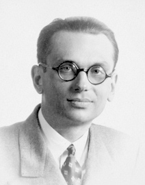
1931年、ベルナイスは自身の集合論に関してクルト・ゲーデルに手紙を送った。ゲーデルはベルナイスの理論を、集合をすべてクラスで置き換え、1ソートで1つの原始概念（帰属関係）からなる理論に簡略化した。ゲーデルはまた、ベルナイスの公理のいくつかを弱め、フォン・ノイマンの選択公理を大域選択公理と等価なものに置き換えた。^{[62][注釈 22]} ゲーデルは、1940年の大域選択と一般連続体仮説の相対的無矛盾性に関するモノグラフの中で、自身の公理系を使った。^[63]

ゲーデルが自身のモノグラフの中で NBG を用いた理由はいくつか考えられる：^{[注釈 23]}

• ゲーデルは数学的理由を与えた—NBGの大域選択公理から、より強い無矛盾な定理が導かれる：「この強い形式の（選択）公理は、他の公理に対して無矛盾であれば、当然弱い形式についての無矛盾性を含意する。」^[5]
• ロバート・ソロヴェイ（英語版）は以下のように予想した：「私が思うに、彼（ゲーデル）は公理的集合論内でモデル理論の基本を発展させることに関連する、細部の議論を避けたかった。」^{[67][注釈 24]}
• ケネス・キューネンはゲーデルが議論を避けた理由を以下のように考えている：「L （構成可能集合）に関する組み合わせ論的アプローチもたくさんある、例えば ... （1940年のモノローグの中でゲーデルは）論理学者以外に説明することを試みていた。 ... このアプローチは L を扱う際に、論理の痕跡を残さないというメリットがある。」^[68]
• チャールズ・パーソンズ (Charles Prsons) はゲーデルの選択に哲学的理由を考えた：「この（「集合の特徴」が集合論の原始概念であるという）見方は、ゲーデルの（モノグラフのように）クラス変数をフレームワークとする理論の選択に反映されているかもしれない。」^[69]

ゲーデルの成果と詳細な説明により、その後20年間にわたって NBG が発展した。^[70] 1963年、ゲーデルの作り上げたNBGの無矛盾性証明を援用して、ポール・コーエンはZFの独立性を証明した。^[71] その後、 ZFC が NBG よりも一般的になった。これにはいくつかの要因があり、その一つは NBG において強制法を扱うには追加の仕事が必要だったためである。^[72] これに関するコーエンの1966年の強制法の発表では、ZFが用いられた。^{[73][注釈 25]} 他の要因としては、NBG が ZFC の保存拡大であることが証明されたからである。^{[注釈 26]}

NBG, ZFC, MK

NBG は論理的に ZFC と等価ではない。なぜなら、NBG の言葉は表現的であるからである。NBG ではクラスに関して表現できる一方、ZFC ではできない。しかし集合に関しては、 NBG も ZFC で同じ内容の表現を含意する。したがって、NBG は ZFC の保存拡大である。 NBG は ZFC が含意しない定理を含意するが、 NBG は保存拡大であるため、これらの定理は真のクラスに関するものでなければならない。例えば、大域選択公理は 真のクラス V は整列可能であり、どの真のクラスも V と一対一対応することを含意するが、これは NBG の定理である。^{[注釈 27]}

保存拡大の帰結の一つは、 ZFC と NBG が無矛盾性同値であることである。 この証明には爆発原理（矛盾からは、何でも証明可能である）を用いる。 ZFC か NBG のいずれかが無矛盾でないと仮定する。すると無矛盾でない理論は集合に関する、矛盾 する表現 ∅ = ∅ かつ ∅ ≠ ∅ を含意する。保存拡大の特性から、もう一方の理論もこれらの表現を含意する。したがって、こちらも無矛盾ではない。ゆえに、 NBG はより表現的であるものの、 ZFC と無矛盾性同値なのである。この結果とフォン・ノイマンの1929年の相対的無矛盾性の証明を合わせると、彼の1925年の公理系にサイズ制限公理を加えたものが ZFC と無矛盾性同値であることが含意される。ZFCはカントール集合論のフレームワークに含まれるため、この事実は完全にこの強力な公理の相対的無矛盾性に関するフォン・ノイマンの懸念を払拭するものである。

NBG は ZFC の保存拡大であるものの、定理は NBG のほうが ZFC より短くエレガントに証明可能である（逆もしかり）。この側面について知られている結果の調査結果は Pudlák 1998 を参照。

モース＝ケリー集合論は、量化子の範囲がクラスである論理式を含む理解の公理型を有する。MK は NBG の無矛盾性を証明できるため、 NBG より強力な理論である一方、^[76]ゲーデルの第二不完全定理から NBG は NBG自身の無矛盾性を証明できない。

NBG に関する存在論的な議論や哲学的な問題、特に ZFC と MK との比較については、Potter 2004の Appendix C を参照。

モデル

ZFC、NBG、MKは累積的階層 V_α および 構成可能階層 L_α の言葉で表現可能なモデルを持つ。 V は到達不能基数 κ を含み、 X が X ⊆ V_κ であると仮定して、 Def(X) は X のパラメータによる1次の定義可能部分集合のクラスを表すとする。記号として "${\displaystyle (X,\in )}$" は領域 ${\displaystyle X}$ と関係 ${\displaystyle \in }$ のモデルを表し、 "${\displaystyle \models }$" は満足関係（en:Structure_(mathematical_logic)#Satisfaction_relation）を表すものとする：

このとき：

• (V_κ, ∈) と (L_κ, ∈) は ZFC のモデルである。^[77]
• (V_κ, V_κ+1, ∈) は MK のモデルであり、ここで V_κ はモデルの集合からなり、 V_κ+1 はモデルのクラスからなる。^[78] MK のモデルは NBG のモデルであるため、このモデルも NBG のモデルである。
• (V_κ, Def(V_κ), ∈) は、NBG の大域選択公理を ZFC の選択公理に置き換えた、メンデルソン版の NBG のモデルである。^[79] (V_κ, ∈) は ZFC のモデルであるため、ZFC 公理はこのモデル内で真である。特に、ZFC の選択公理が成り立つが、 NBG の大域選択公理は成り立たないかもしれない。^{[注釈 28]} 存在を主張するクラスは1次の定義で定義できることから、NBG のクラス存在公理はこのモデル内で真である。例えば、 ${\displaystyle E}$ が以下のように定義されるため、帰属公理が成り立つ：
  $${\displaystyle E=\{x\in V_{\kappa }:(V_{\kappa },\in )\models \exists u\ \exists v[x=(u,v)\land u\in v]\}.}$$

  
• (L_κ, L_κ⁺, ∈) （κ⁺ は κ の後続基数）は NBG のモデルである。^{[注釈 29]} NBG のクラス存在公理は (L_κ, L_κ⁺, ∈) の中で真である。例えば、 ${\displaystyle E}$ が以下のように定義されるため、帰属公理が成り立つ：
  $${\displaystyle E=\{x\in L_{\kappa }:(L_{\kappa },\in )\models \exists u\ \exists v[x=(u,v)\land u\in v]\}.}$$

  
  ゆえに、 E ∈ 𝒫(L_κ) である。一般連続体仮説が L の中で真というゲーデルの証明において、ゲーデルは 𝒫(L_κ) ⊆ L_κ⁺ であることを証明した。^[81] したがって、 E ∈ L_κ⁺ であり、ゆえに (L_κ, L_κ⁺, ∈) の中で帰属公理は真である。同様に、ほかのクラス存在公理も真である。（順序数のクラスを構成可能集合に移す）ゲーデルの関数を κ 未満の順序数に制限することによって L_κ が整列可能であるため、大域選択公理は真である。したがって、 (L_κ, L_κ⁺, ∈) は NBG のモデルである。

圏論

NBG の基本概念体系は「大きな対象」をパラドックスのおそれなしに議論する足場を提供する。例えば、圏論の進展において、「大きい圏」は対象と射が真のクラスをなす圏として定義される。一方、「小さな圏」は対象と射が集合の要素になる圏である。このように、NBG で大きな圏を扱えるため、「すべての集合の圏」や「すべての小さい圏の圏」をパラドックスのおそれなしに議論できる。

しかし、NBG は「すべての圏の圏」を扱えない。大きな圏は「すべての圏の圏」の要素となりえて、かつ NBG は真のクラスが何かの要素になることを許容していないためである。このような「圏」を形式的に議論するための基本概念体系の一つの拡張がクラスの集まりとしての複合体(conglomerate)である。このとき「すべての圏の圏」は、すべての圏からなる複合体を対象全体とし、A と B が対象全体を動くときに A から B へのすべての射からなる複合体^[82]を射の全体として定義される。 圏論のためにクラスを集合と同様の基本概念体系に含めるのが妥当であるのかどうかについては、 Muller 2001 を参照せよ。

脚注

注釈

出典

参考文献

• Adámek, Jiří; Herrlich, Horst; Strecker, George E. (1990), Abstract and Concrete Categories (The Joy of Cats) (1st ed.), New York: Wiley & Sons, ISBN 978-0-471-60922-3, http://katmat.math.uni-bremen.de/acc/ .
  • Adámek, Jiří; Herrlich, Horst; Strecker, George E. (2004) [1990], Abstract and Concrete Categories (The Joy of Cats) (Dover ed.), New York: Dover Publications, ISBN 978-0-486-46934-8, http://katmat.math.uni-bremen.de/acc/ .
• Bernays, Paul (1937), “A System of Axiomatic Set Theory—Part I”, The Journal of Symbolic Logic 2 (1): 65–77, doi:10.2307/2268862, JSTOR 2268862, https://jstor.org/stable/2268862 .
• Bernays, Paul (1941), “A System of Axiomatic Set Theory—Part II”, The Journal of Symbolic Logic 6 (1): 1–17, doi:10.2307/2267281, JSTOR 2267281, https://jstor.org/stable/2267281 .
• Bernays, Paul (1991), Axiomatic Set Theory (2nd Revised ed.), Dover Publications, ISBN 978-0-486-66637-2 .
• Bourbaki, Nicolas (2004), Elements of Mathematics: Theory of Sets, Springer, ISBN 978-3-540-22525-6, https://archive.org/details/springer_10.1007-978-3-642-59309-3 .
• Chuaqui, Rolando (1981), Axiomatic Set Theory: Impredicative Theories of Classes, North-Holland, ISBN 0-444-86178-5 .
• Cohen, Paul (1963), “The Independence of the Continuum Hypothesis”, Proceedings of the National Academy of Sciences of the United States of America 50 (6): 1143–1148, Bibcode: 1963PNAS...50.1143C, doi:10.1073/pnas.50.6.1143, PMC 221287, PMID 16578557, http://www.pubmedcentral.nih.gov/articlerender.fcgi?tool=pmcentrez&artid=221287 .
• Cohen, Paul (1966), Set Theory and the Continuum Hypothesis, W. A. Benjamin .
  • Cohen, Paul (2008), Set Theory and the Continuum Hypothesis, Dover Publications, ISBN 978-0-486-46921-8, https://books.google.com/books?id=Z4NCAwAAQBAJ .
• Dawson, John W. (1997), Logical dilemmas: The life and work of Kurt Gödel, Wellesley, MA: AK Peters .
• Easton, William B. (1964), Powers of Regular Cardinals (PhD thesis), Princeton University .
• Felgner, Ulrich (1971), “Comparison of the axioms of local and universal choice”, Fundamenta Mathematicae 71: 43–62, doi:10.4064/fm-71-1-43-62, http://matwbn.icm.edu.pl/ksiazki/fm/fm71/fm7113.pdf .
• Ferreirós, José (2007), Labyrinth of Thought: A History of Set Theory and Its Role in Mathematical Thought (2nd revised ed.), Basel, Switzerland: Birkhäuser, ISBN 978-3-7643-8349-7 .
• Gödel, Kurt (1940), The Consistency of the Axiom of Choice and of the Generalized Continuum Hypothesis with the Axioms of Set Theory (Revised ed.), Princeton University Press, ISBN 978-0-691-07927-1 .
  • Gödel, Kurt (2008), The Consistency of the Axiom of Choice and of the Generalized Continuum Hypothesis with the Axioms of Set Theory, with a foreword by Laver, Richard (Paperback ed.), Ishi Press, ISBN 978-0-923891-53-4 .
• Gödel, Kurt (1986), Collected Works, Volume 1: Publications 1929–1936, Oxford University Press, ISBN 978-0-19-514720-9 .
• Gödel, Kurt (1990), Collected Works, Volume 2: Publications 1938–1974, Oxford University Press, ISBN 978-0-19-514721-6 .
• Gödel, Kurt (2003), Collected Works, Volume 4: Correspondence A–G, Oxford University Press, ISBN 978-0-19-850073-5 .
• Gray, Robert (1991), “Computer programs and mathematical proofs”, The Mathematical Intelligencer 13 (4): 45–48, doi:10.1007/BF03028342 .
• Hallett, Michael (1984), Cantorian Set Theory and Limitation of Size (Hardcover ed.), Oxford: Clarendon Press, ISBN 978-0-19-853179-1 .
  • Hallett, Michael (1986), Cantorian Set Theory and Limitation of Size (Paperback ed.), Oxford: Clarendon Press, ISBN 978-0-19-853283-5 .
• Kanamori, Akihiro (2009b), The Higher Infinite: Large Cardinals in Set Theory from Their Beginnings, Springer, ISBN 978-3-540-88867-3 .
• Kanamori, Akihiro (2009), “Bernays and Set Theory”, Bulletin of Symbolic Logic 15 (1): 43–69, doi:10.2178/bsl/1231081769, JSTOR 25470304, http://math.bu.edu/people/aki/17a.pdf .
• Kanamori, Akihiro (2012), “In Praise of Replacement”, Bulletin of Symbolic Logic 18 (1): 46–90, doi:10.2178/bsl/1327328439, JSTOR 41472440, http://math.bu.edu/people/aki/20.pdf .
• Kunen, Kenneth (1980), Set Theory: An Introduction to Independence Proofs (Hardcover ed.), North-Holland, ISBN 978-0-444-86839-8 .
  • Kunen, Kenneth (2012), Set Theory: An Introduction to Independence Proofs (Paperback ed.), North-Holland, ISBN 978-0-444-56402-3 .
• Mendelson, Elliott (1997), An Introduction to Mathematical Logic (4th ed.), London: Chapman and Hall/CRC, ISBN 978-0-412-80830-2 . - Pp. 225–86 contain the classic textbook treatment of NBG, showing how it does what we expect of set theory, by grounding relations, order theory, ordinal numbers, transfinite numbers, etc.
• Mirimanoff, Dmitry (1917), “Les antinomies de Russell et de Burali-Forti et le problème fondamental de la théorie des ensembles”, L'Enseignement Mathématique 19: 37–52 .
• Montague, Richard (1961), “Semantic Closure and Non-Finite Axiomatizability I”, in Buss, Samuel R., Infinitistic Methods: Proceedings of the Symposium on Foundations of Mathematics, Pergamon Press, pp. 45–69 .
• Mostowski, Andrzej (1950), “Some impredicative definitions in the axiomatic set theory”, Fundamenta Mathematicae 37: 111–124, doi:10.4064/fm-37-1-111-124, http://matwbn.icm.edu.pl/ksiazki/fm/fm37/fm37110.pdf .
• Muller, F. A. (1 September 2001), “Sets, classes, and categories”, British Journal for the Philosophy of Science 52 (3): 539–73, doi:10.1093/bjps/52.3.539, http://philsci-archive.pitt.edu/1372/1/SetClassCat.PDF .
• Müller, Gurt, ed. (1976), Sets and Classes: On the Work of Paul Bernays, Studies in Logic and the Foundations of Mathematics Volume 84, Amsterdam: North Holland, ISBN 978-0-7204-2284-9 .
• Potter, Michael (2004), Set Theory and Its Philosophy: A Critical Introduction (Hardcover ed.), Oxford University Press, ISBN 978-0-19-926973-0 .
  • Potter, Michael (2004p), Set Theory and Its Philosophy: A Critical Introduction (Paperback ed.), Oxford University Press, ISBN 978-0-19-927041-5 .
• Pudlák, Pavel (1998), “The Lengths of Proofs”, in Buss, Samuel R., Handbook of Proof Theory, Elsevier, pp. 547–637, ISBN 978-0-444-89840-1, http://users.math.cas.cz/~pudlak/length.pdf .
• Smullyan, Raymond M.; Fitting, Melvin (2010) [Revised and corrected edition: first published in 1996 by Oxford University Press], Set Theory and the Continuum Problem, Dover, ISBN 978-0-486-47484-7 .
• Solovay, Robert M. (1990), “Introductory note to 1938, 1939, 1939a and 1940”, Kurt Gödel Collected Works, Volume 2: Publications 1938–1974, Oxford University Press, pp. 1–25, ISBN 978-0-19-514721-6 .
• von Neumann, John (1922), “Zur Einführung der transfiniten Zahlen”, Acta Litt. Acad. Sc. Szeged X. 1: 199–208, http://bbi-math.narod.ru/newmann/newmann.html .
  • English translation: van Heijenoort, Jean (2002a) [1967], “On the introduction of transfinite numbers”, From Frege to Gödel: A Source Book in Mathematical Logic, 1879-1931 (Fourth Printing ed.), Harvard University Press, pp. 346–354, ISBN 978-0-674-32449-7, https://books.google.com/books?id=v4tBTBlU05sC&pg=PA346 .
  • English translation: van Heijenoort, Jean (2002b) [1967], “An axiomatization of set theory”, From Frege to Gödel: A Source Book in Mathematical Logic, 1879-1931 (Fourth Printing ed.), Harvard University Press, pp. 393–413, ISBN 978-0-674-32449-7, https://books.google.com/books?id=v4tBTBlU05sC&pg=PA393 .
• von Neumann, John (1925), “Eine Axiomatisierung der Mengenlehre”, Journal für die Reine und Angewandte Mathematik 154: 219–240, http://gdz.sub.uni-goettingen.de/dms/load/img/?PPN=PPN243919689_0154&DMDID=DMDLOG_0025 .
• von Neumann, John (1928), “Die Axiomatisierung der Mengenlehre”, Mathematische Zeitschrift 27: 669–752, doi:10.1007/bf01171122, http://gdz.sub.uni-goettingen.de/dms/load/img/?PPN=PPN266833020_0027&DMDID=DMDLOG_0042 .
• von Neumann, John (1929), “Über eine Widerspruchsfreiheitsfrage in der axiomatischen Mengenlehre”, Journal für die Reine und Angewandte Mathematik 160: 227–241, http://gdz.sub.uni-goettingen.de/dms/load/img/?PPN=PPN243919689_0160&DMDID=DMDLOG_0019 .

外部リンク

• Szudzik, Matthew. "von Neumann-Bernays-Gödel Set Theory". mathworld.wolfram.com (英語).