Feigenbaum function

In the study of dynamical systems the term Feigenbaum function has been used to describe two different functions introduced by the physicist Mitchell Feigenbaum:^[1]

• the solution to the Feigenbaum-Cvitanović functional equation; and
• the scaling function that described the covers of the attractor of the logistic map

Idea

Period-doubling route to chaos

In the logistic map,

${\displaystyle x_{n+1}=rx_{n}(1-x_{n}),}$

(1)

we have a function ${\displaystyle f_{r}(x)=rx(1-x)}$, and we want to study what happens when we iterate the map many times. The map might fall into a fixed point, a fixed cycle, or chaos. When the map falls into a stable fixed cycle of length ${\displaystyle n}$, we would find that the graph of ${\displaystyle f_{r}^{n}}$ and the graph of ${\displaystyle x\mapsto x}$ intersects at ${\displaystyle n}$ points, and the slope of the graph of ${\displaystyle f_{r}^{n}}$ is bounded in ${\displaystyle (-1,+1)}$ at those intersections.

For example, when ${\displaystyle r=3.0}$, we have a single intersection, with slope bounded in ${\displaystyle (-1,+1)}$, indicating that it is a stable single fixed point.

As ${\displaystyle r}$ increases to beyond ${\displaystyle r=3.0}$, the intersection point splits to two, which is a period doubling. For example, when ${\displaystyle r=3.4}$, there are three intersection points, with the middle one unstable, and the two others stable.

As ${\displaystyle r}$ approaches ${\displaystyle r=3.45}$, another period-doubling occurs in the same way. The period-doublings occur more and more frequently, until at a certain ${\displaystyle r\approx 3.56994567}$, the period doublings become infinite, and the map becomes chaotic. This is the period-doubling route to chaos.

Scaling limit

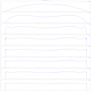
Looking at the images, one can notice that at the point of chaos ${\displaystyle r^{*}=3.5699\cdots }$, the curve of ${\displaystyle f_{r^{*}}^{\infty }}$ looks like a fractal. Furthermore, as we repeat the period-doublings${\displaystyle f_{r^{*}}^{1},f_{r^{*}}^{2},f_{r^{*}}^{4},f_{r^{*}}^{8},f_{r^{*}}^{16},\dots }$, the graphs seem to resemble each other, except that they are shrunken towards the middle, and rotated by 180 degrees.

This suggests to us a scaling limit: if we repeatedly double the function, then scale it up by ${\displaystyle \alpha }$ for a certain constant ${\displaystyle \alpha }$:

then at the limit, we would end up with a function ${\displaystyle g}$ that satisfies ${\displaystyle g(x)=-\alpha g(g(-x/\alpha ))}$. Further, as the period-doubling intervals become shorter and shorter, the ratio between two period-doubling intervals converges to a limit, the first Feigenbaum constant ${\displaystyle \delta =4.6692016\cdots }$.

The constant ${\displaystyle \alpha }$ can be numerically found by trying many possible values. For the wrong values, the map does not converge to a limit, but when it is ${\displaystyle \alpha =2.5029\dots }$, it converges. This is the second Feigenbaum constant.

Chaotic regime

In the chaotic regime, ${\displaystyle f_{r}^{\infty }}$, the limit of the iterates of the map, becomes chaotic dark bands interspersed with non-chaotic bright bands.

Other scaling limits

When ${\displaystyle r}$ approaches ${\displaystyle r\approx 3.8494344}$, we have another period-doubling approach to chaos, but this time with periods 3, 6, 12, ... This again has the same Feigenbaum constants ${\displaystyle \delta ,\alpha }$. The limit of ${\textstyle f(x)\mapsto -\alpha f(f(-x/\alpha ))}$ is also the same function. This is an example of universality.

We can also consider period-tripling route to chaos by picking a sequence of ${\displaystyle r_{1},r_{2},\dots }$ such that ${\displaystyle r_{n}}$ is the lowest value in the period-${\displaystyle 3^{n}}$ window of the bifurcation diagram. For example, we have ${\displaystyle r_{1}=3.8284,r_{2}=3.85361,\dots }$, with the limit ${\displaystyle r_{\infty }=3.854077963\dots }$. This has a different pair of Feigenbaum constants ${\displaystyle \delta =55.26\dots ,\alpha =9.277\dots }$.^[2] And ${\displaystyle f_{r}^{\infty }}$converges to the fixed point to

As another example, period-4-pling has a pair of Feigenbaum constants distinct from that of period-doubling, even though period-4-pling is reached by two period-doublings. In detail, define ${\displaystyle r_{1},r_{2},\dots }$ such that ${\displaystyle r_{n}}$ is the lowest value in the period-${\displaystyle 4^{n}}$ window of the bifurcation diagram. Then we have ${\displaystyle r_{1}=3.960102,r_{2}=3.9615554,\dots }$, with the limit ${\displaystyle r_{\infty }=3.96155658717\dots }$. This has a different pair of Feigenbaum constants ${\displaystyle \delta =981.6\dots ,\alpha =38.82\dots }$.

In general, each period-multiplying route to chaos has its own pair of Feigenbaum constants. In fact, there are typically more than one. For example, for period-7-pling, there are at least 9 different pairs of Feigenbaum constants.^[2]

Generally, ${\textstyle 3\delta \approx 2\alpha ^{2}}$, and the relation becomes exact as both numbers increase to infinity: ${\displaystyle \lim \delta /\alpha ^{2}=2/3}$.

Feigenbaum-Cvitanović functional equation

This functional equation arises in the study of one-dimensional maps that, as a function of a parameter, go through a period-doubling cascade. Discovered by Mitchell Feigenbaum and Predrag Cvitanović,^[3] the equation is the mathematical expression of the universality of period doubling. It specifies a function g and a parameter α by the relation

${\displaystyle g(x)=-\alpha g(g(-x/\alpha ))}$

with the initial conditions

For a particular form of solution with a quadratic dependence of the solution near x = 0, α = 2.5029... is one of the Feigenbaum constants.

The power series of ${\displaystyle g}$ is approximately^[4]

Renormalization

The Feigenbaum function can be derived by a renormalization argument.^[5]

The Feigenbaum function satisfies^[6]

for any map on the real line ${\displaystyle F}$ at the onset of chaos.

Scaling function

The Feigenbaum scaling function provides a complete description of the attractor of the logistic map at the end of the period-doubling cascade. The attractor is a Cantor set, and just as the middle-third Cantor set, it can be covered by a finite set of segments, all bigger than a minimal size d_n. For a fixed d_n the set of segments forms a cover Δ_n of the attractor. The ratio of segments from two consecutive covers, Δ_n and Δ_n+1 can be arranged to approximate a function σ, the Feigenbaum scaling function.

See also

• Logistic map
• Presentation function

Notes

Bibliography

• Feigenbaum, M. (1978). "Quantitative universality for a class of nonlinear transformations". Journal of Statistical Physics. 19 (1): 25–52. Bibcode:1978JSP....19...25F. CiteSeerX 10.1.1.418.9339. doi:10.1007/BF01020332. MR 0501179. S2CID 124498882.
• Feigenbaum, M. (1979). "The universal metric properties of non-linear transformations". Journal of Statistical Physics. 21 (6): 669–706. Bibcode:1979JSP....21..669F. CiteSeerX 10.1.1.418.7733. doi:10.1007/BF01107909. MR 0555919. S2CID 17956295.
• Feigenbaum, Mitchell J. (1980). "The transition to aperiodic behavior in turbulent systems". Communications in Mathematical Physics. 77 (1): 65–86. Bibcode:1980CMaPh..77...65F. doi:10.1007/BF01205039. S2CID 18314876.
• Epstein, H.; Lascoux, J. (1981). "Analyticity properties of the Feigenbaum Function". Commun. Math. Phys. 81 (3): 437–453. Bibcode:1981CMaPh..81..437E. doi:10.1007/BF01209078. S2CID 119924349.
• Feigenbaum, Mitchell J. (1983). "Universal Behavior in Nonlinear Systems". Physica. 7D (1–3): 16–39. Bibcode:1983PhyD....7...16F. doi:10.1016/0167-2789(83)90112-4. Bound as Order in Chaos, Proceedings of the International Conference on Order and Chaos held at the Center for Nonlinear Studies, Los Alamos, New Mexico 87545, USA 24–28 May 1982, Eds. David Campbell, Harvey Rose; North-Holland Amsterdam ISBN 0-444-86727-9.
• Lanford III, Oscar E. (1982). "A computer-assisted proof of the Feigenbaum conjectures". Bull. Am. Math. Soc. 6 (3): 427–434. doi:10.1090/S0273-0979-1982-15008-X. MR 0648529.
• Campanino, M.; Epstein, H.; Ruelle, D. (1982). "On Feigenbaums functional equation ${\displaystyle g\circ g(\lambda x)+\lambda g(x)=0}$". Topology. 21 (2): 125–129. doi:10.1016/0040-9383(82)90001-5. MR 0641996.
• Lanford III, Oscar E. (1984). "A shorter proof of the existence of the Feigenbaum fixed point". Commun. Math. Phys. 96 (4): 521–538. Bibcode:1984CMaPh..96..521L. CiteSeerX 10.1.1.434.1465. doi:10.1007/BF01212533. S2CID 121613330.
• Epstein, H. (1986). "New proofs of the existence of the Feigenbaum functions" (PDF). Commun. Math. Phys. 106 (3): 395–426. Bibcode:1986CMaPh.106..395E. doi:10.1007/BF01207254. S2CID 119901937.
• Eckmann, Jean-Pierre; Wittwer, Peter (1987). "A complete proof of the Feigenbaum Conjectures". J. Stat. Phys. 46 (3/4): 455. Bibcode:1987JSP....46..455E. doi:10.1007/BF01013368. MR 0883539. S2CID 121353606.
• Stephenson, John; Wang, Yong (1991). "Relationships between the solutions of Feigenbaum's equation". Appl. Math. Lett. 4 (3): 37–39. doi:10.1016/0893-9659(91)90031-P. MR 1101871.
• Stephenson, John; Wang, Yong (1991). "Relationships between eigenfunctions associated with solutions of Feigenbaum's equation". Appl. Math. Lett. 4 (3): 53–56. doi:10.1016/0893-9659(91)90035-T. MR 1101875.
• Briggs, Keith (1991). "A precise calculation of the Feigenbaum constants". Math. Comp. 57 (195): 435–439. Bibcode:1991MaCom..57..435B. doi:10.1090/S0025-5718-1991-1079009-6. MR 1079009.
• Tsygvintsev, Alexei V.; Mestel, Ben D.; Obaldestin, Andrew H. (2002). "Continued fractions and solutions of the Feigenbaum-Cvitanović equation". Comptes Rendus de l'Académie des Sciences, Série I. 334 (8): 683–688. doi:10.1016/S1631-073X(02)02330-0.
• Mathar, Richard J. (2010). "Chebyshev series representation of Feigenbaum's period-doubling function". arXiv:1008.4608 [math.DS].
• Varin, V. P. (2011). "Spectral properties of the period-doubling operator". KIAM Preprint. 9. arXiv:1202.4672.
• Weisstein, Eric W. "Feigenbaum Function". MathWorld.